Perturb for Instruments

Perturb tells you which parts of an observation an answer depends on. That is exactly what you need to know when designing an instrument: keep the parts that matter, drop the rest.

This demo uses the same toy spectrum and least-squares fit as Perturb for Observations, but asks a different question: what is the smallest instrument that still measures every parameter almost as well as the full one? Perturb scores every data point, the least useful one is removed, and the loop repeats.

import perturb as pt
from perturb import plotting

The available instrumentation

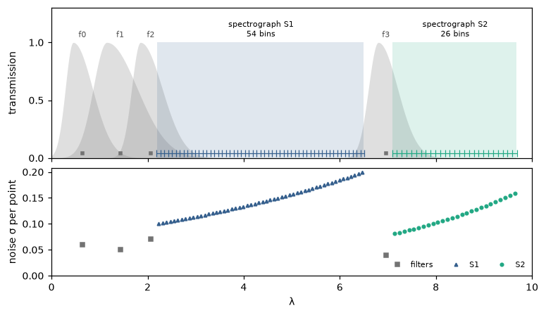
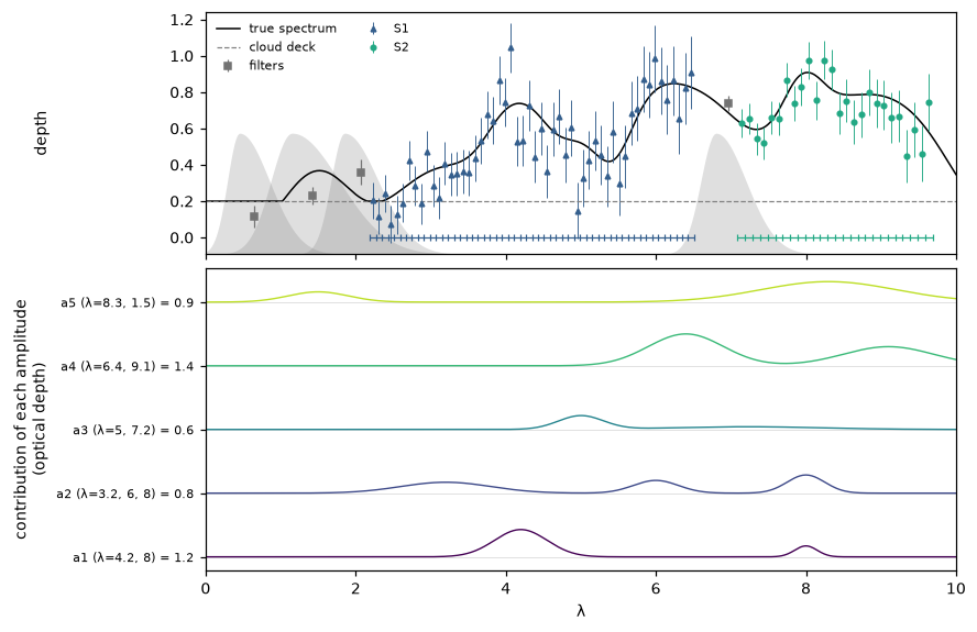
Everything the instrument could carry: 4 overlapping filters, which can each be kept or dropped, and two spectrographs, S1 and S2, which can be cropped from either end or have neighbouring bins merged (lower resolution, but less noise).

The spectrum

The spectrum is set by 5 unknown amplitudes, each with bands in more than one place, so most can be read from more than one instrument. This time the design has to serve all five.

The black box

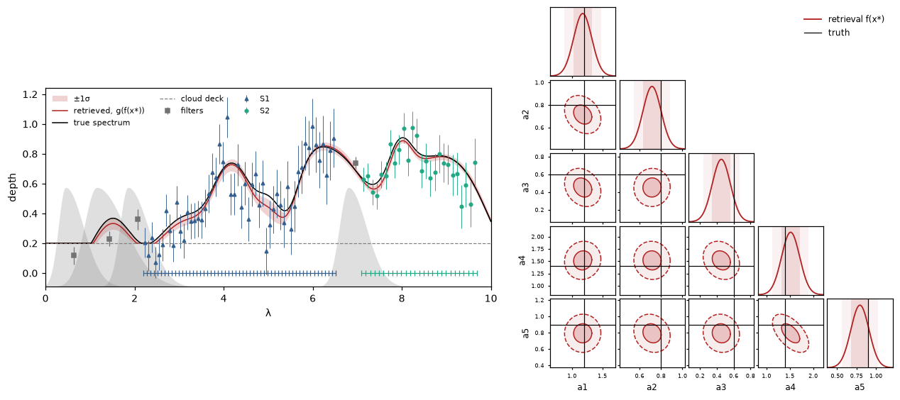
f fits the 5 amplitudes by least squares. The widths of the posteriors on the right are what the design loop tries to keep.

Steps 1 and 2: kernel width and how far to perturb

These work just as in the other demos. Every design step below reuses this kernel width.

fit = pt.fit_kernel_width(X_prior, obs["x_axis"], normalise=True)
FWHM = fit["fwhm"]

perturber = pt.Perturber(f, obs["x_axis"], obs["sigma"], FWHM, scale="own", batch_size=1)
wide = perturber(obs["y"], pt.magnitude_grid(xi_max=5, n=41))
XI_MAX = pt.max_magnitude(pt.in_distribution_curve(wide, forward, tol=0.2))

kernel FWHM = 1.521 ± 0.016 in λ
in distribution up to |xi| = 0.75 sigma

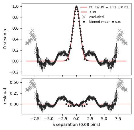
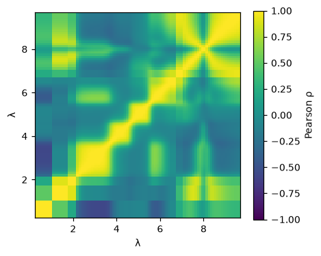
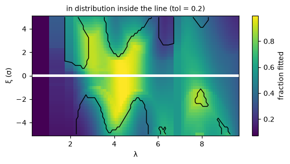
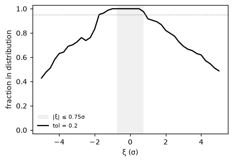
With this much noise even a modest nudge is large next to the signal: deep bands saturate and amplitudes hit their limits, so the fit can only be trusted out to 0.75σ.

Step 3: perturb the observation

Each nudge costs one least-squares fit, so 21 nudge sizes keep a run to a few seconds.

result = perturber(obs["y"], pt.magnitude_grid(xi_max=XI_MAX, n=21))

Step 4: visualise

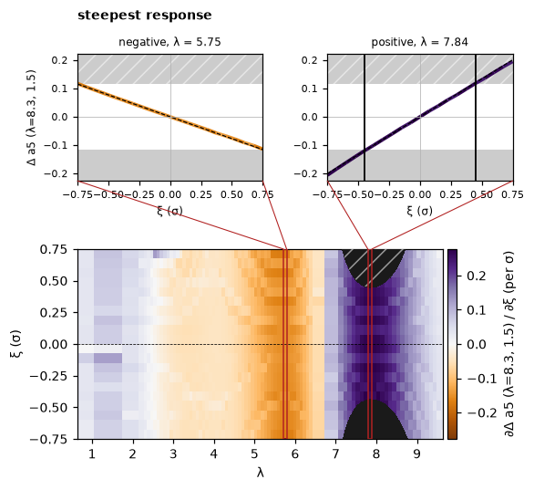
Response-gradient maps for a4 and a5. Each amplitude is read from under its own bands (purple), and pushed the other way by its neighbours’ bands (orange): raise the spectrum next door, and the neighbouring amplitude takes the credit.

plotting.gradient_map(result, output=3)
plotting.gradient_map(result, output=4)

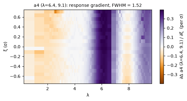
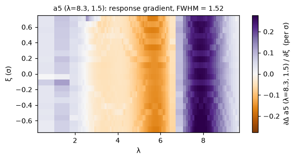
With threshold set to a5’s own error bar, the callouts black out any region where a nudge of under a σ already moves a5 by more than its uncertainty.

plotting.callouts(result, output=4, threshold=sigma_retrieved[4], n_positive=1, n_negative=1, n_nonlinear=0)

Step 5: designing the instrument

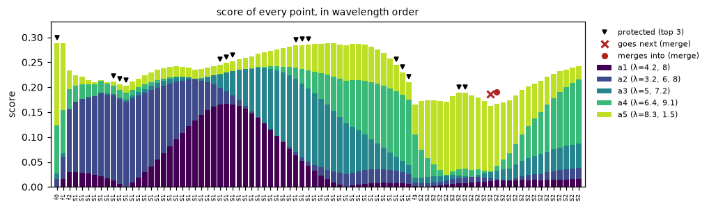
Divide each point’s importance by the parameter’s error bar, and you get a score: how far the answer moves, in its own error bars, when that region moves by its noise. Then, one point per step:

1. Each parameter protects its 3 highest-scoring points, so nothing one parameter relies on is lost because the others don’t need it.
2. The unprotected point with the lowest total score goes: a filter is dropped, a spectrograph’s end bin is cropped, or an interior bin is merged with its neighbour.
3. Refit, re-run Perturb on the smaller instrument, and repeat, all the way down to nothing.

Here are the scores at the very first step, for the full instrument. The colours stack each amplitude’s score, the triangles mark protected points, and the red cross is the first point to go: an S2 bin, merged into its neighbour.

for step in range(len(obs["y"])):
    o = observe(config)                                  # the current instrument's observation
    fo = retrieval(o)
    r = pt.Perturber(fo, o["x_axis"], o["sigma"], FWHM, scale="own", batch_size=1)(
        o["y"], pt.magnitude_grid(XI_MAX, 21))
    score = np.abs(r.importance) / sigma_retrieved       # what each point is worth, per parameter
    config = design_step(config, o, score, k=3)          # protect the top 3, remove the weakest

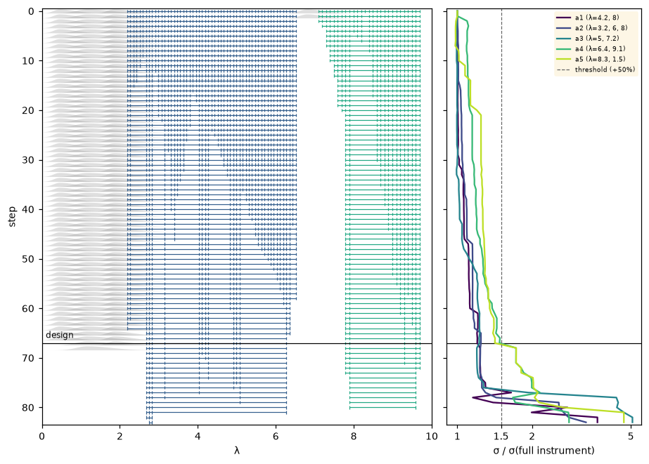
84 steps to no points; design after 67 steps: 84 -> 17 points

Left: how the instrument shrinks, one row per step (filter profiles in grey, spectrograph bins as ticks). Right: each amplitude’s error bar relative to the full instrument’s. The chosen design is the smallest instrument that keeps every parameter within 50% of its original precision.

The design next to the full instrument

The design keeps 17 of the 84 data points and still constrains all five amplitudes (red) almost as well as the full instrument (grey).

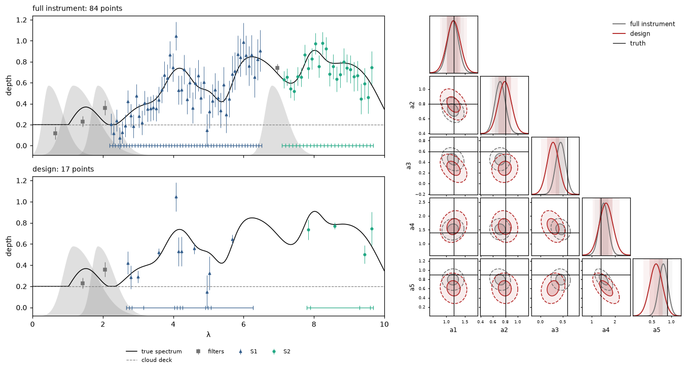
A point’s score includes its neighbours, since Perturb nudges a whole region at once, so the loop removes points in the order their neighbourhood stops mattering. And like any single run, this design is tied to one truth and noise draw; for real planning, repeat it over plausible ones.

Using it on your own retrieval

import perturb as pt
from perturb import plotting

fit = pt.fit_kernel_width(X_prior, x_axis)                                          # 1. kernel width
perturber = pt.Perturber(f, x_axis, sigma, fit["fwhm"], scale="own", batch_size=1)  # f: one fit per call
wide = perturber(x, pt.magnitude_grid(5, 41))                                       #    explore
xi_max = pt.max_magnitude(pt.in_distribution_curve(wide, forward, tol=0.1))         # 2. how far
result = perturber(x, pt.magnitude_grid(xi_max, 21))                                # 3. perturb
plotting.gradient_map(result, output=0)                                             # 4. plot
score = np.abs(result.importance) / sigma_retrieved                                 # 5. what each point is worth