Perturb for Observations | Gaussian Perturb

Perturb is usually used to ask what does this answer depend on? Here we read it backwards, as a requirement:

We want to measure one parameter to ±0.1. How noisy can each data point be before it moves the answer by more than that, and how many exposures does each instrument need to get there?

The black box this time is not a neural network but a plain least-squares fit. Perturb doesn’t mind: all it needs is observations in and answers out.

The idea is simple. Nudge each region of the observation by a growing multiple of its noise, and note the first nudge size that moves the answer by more than the target. That is how much noise the region can tolerate. Averaging N exposures divides the noise by √N, which turns it into a number of exposures.

import perturb as pt
from perturb import plotting

The instrument

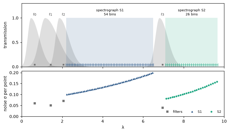
A toy spectrum is observed by 4 overlapping photometric filters and two spectrographs, S1 and S2. Top: what each one covers. Bottom: the noise of every data point.

Transmission of the four filters and the bins of the two spectrographs (top), and the noise of every data point (bottom)

The spectrum and the target

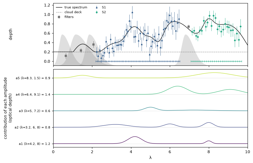
The spectrum is set by 5 unknown amplitudes, each controlling bands in two or three places, which overlap so that neighbouring amplitudes can partly trade off against each other. We want to pin down a4, which has one band at the red end of S1 and one in S2. Bottom: the spectrum taken apart into each amplitude’s contribution.

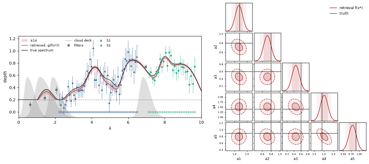
The observed spectrum with error bars (top), and each amplitude's contribution drawn separately (bottom)

The black box

f fits the 5 amplitudes to an observation by least squares. One exposure of everything gets a4 to ±0.195, about twice the target.

Left: the true and retrieved spectrum. Right: a corner plot of the retrieved amplitudes against the truth

Step 1: the width of the kernel

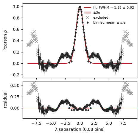
As before, Perturb nudges a smooth neighbourhood rather than single points. Here the overall depth of the spectra varies far more than their shape, so each prior spectrum is normalised first (normalise=True).

fit = pt.fit_kernel_width(X_prior, obs["x_axis"], normalise=True)
FWHM = fit["fwhm"]
plotting.kernel_fit(fit)
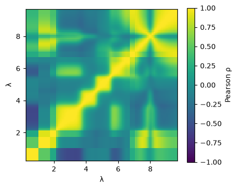
plotting.correlation_matrix(fit)

kernel FWHM = 1.521 ± 0.016 in λ

Correlation between pairs of points against their separation in wavelength, with a Gaussian fit

Correlation matrix of every data point: coarse cells for the filters, fine ones for the spectrographs

Step 2: how far to perturb

Two settings matter for a real instrument. The noise jumps between filters and spectrograph bins, so each point is nudged by its own noise (scale="own"). And a least-squares fit takes one observation at a time (batch_size=1).

perturber = pt.Perturber(f, obs["x_axis"], obs["sigma"], FWHM, scale="own", batch_size=1)
wide = perturber(obs["y"], pt.magnitude_grid(xi_max=5, n=41))
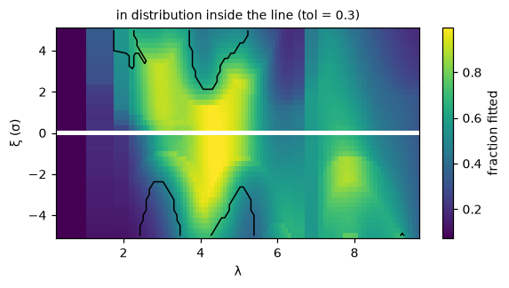
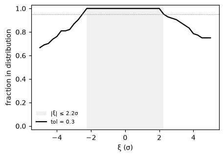
curve = pt.in_distribution_curve(wide, forward, tol=0.3)
plotting.ood_map(curve, wide)

Map of the fit's response for every position and nudge size, with the trusted region outlined

XI_MAX = pt.max_magnitude(curve)
plotting.in_distribution(curve)

in distribution up to |xi| = 2.25 sigma

Fraction of positions still trusted against nudge size

Step 3: perturb the observation

To find where each response crosses the target we need a fine grid of nudge sizes, in steps of 0.1σ.

result = perturber(obs["y"], pt.magnitude_grid(XI_MAX, 47))

Step 4: the response against the target

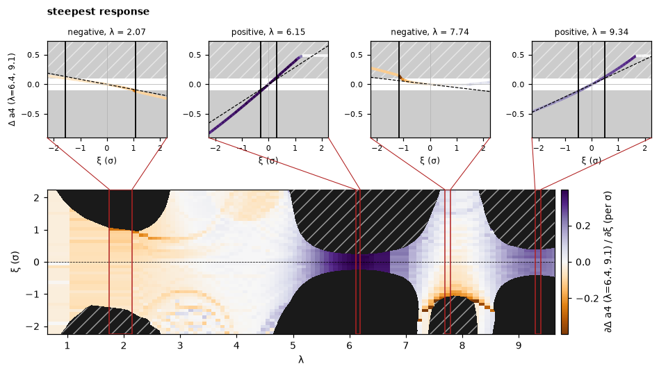
With threshold set to the target, every response bigger than ±0.1 is blacked out. The blacked-out areas are the regions where a single exposure isn’t good enough.

plotting.callouts(result, output=3, threshold=0.1, n_positive=2, n_negative=2, n_nonlinear=0)

Response-gradient map for a4 with the four steepest responses called out, and responses beyond the target blacked out

Step 5: the noise budget

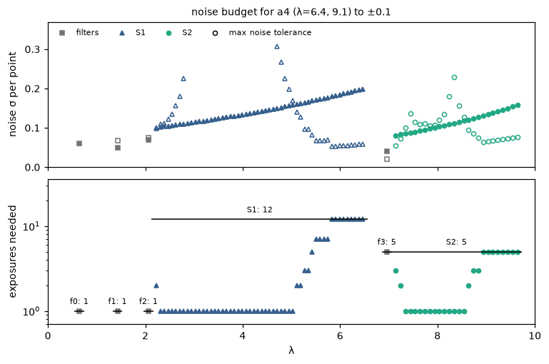
result.crossing(target) gives, for every position, the first nudge size (below and above zero) at which the answer moves by the target. Taking the nearer one gives each point’s largest allowed noise, and from that the number of exposures it needs. A spectrograph reads all its bins in one exposure, so it needs as many as its most demanding bin.

cross = result.crossing(0.1)[:, :, 3]                       # for a4
xi_c = np.fmin(np.abs(cross[:, 0]), np.abs(cross[:, 1]))    # the nearer side
allowed = xi_c * obs["sigma"]                               # largest noise each point can have
need = np.where(np.isnan(xi_c), 1, np.ceil(1 / xi_c**2))    # exposures each point needs

instrument points crossed tightest allowed noise exposures
        f0      1       0                    any         1
        f1      1       1                 0.0685         1
        f2      1       1                 0.0753         1
        S1     54      31                 0.0527        12
        f3      1       1                 0.0196         5
        S2     26      26                 0.0554         5
25 exposures in all

Top: each point’s noise now (filled) and the most it can have (open). Bottom: the exposures each point needs, with each instrument’s line at the number it gets.

Current against allowed noise for every point (top), and the number of exposures needed per point and per instrument (bottom)

Checking the plan

Take that many exposures of each instrument and refit. The plan gets a4 to ±0.081, inside the ±0.1 target.

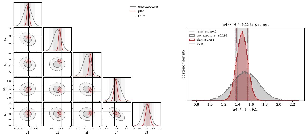
Corner plots of one exposure against the plan (left), and the posterior of a4 for each, with the plan inside the required band (right)

It beats the target with room to spare because the budget is deliberately strict: it asks that no whole region, moving together by its noise, shifts the answer too far. Independent noise in each bin partly cancels out, so treat the budget as exact for noise that drifts smoothly with wavelength (a systematic, say) and as a safe upper bound for white noise. It is also tied to this one truth and noise draw; for real planning, repeat it over plausible ones.

Using it on your own retrieval

import perturb as pt

fit = pt.fit_kernel_width(X_prior, x_axis)                                          # 1. kernel width
perturber = pt.Perturber(f, x_axis, sigma, fit["fwhm"], scale="own", batch_size=1)
xi_max = pt.max_magnitude(pt.in_distribution_curve(perturber(x, pt.magnitude_grid(5, 41)), forward))  # 2. how far
result = perturber(x, pt.magnitude_grid(xi_max, 61))                                # 3. perturb
cross = result.crossing(target)[:, :, p]                                            # 4. where it crosses
xi_c = np.fmin(np.abs(cross[:, 0]), np.abs(cross[:, 1]))
allowed = xi_c * sigma                                                              # 5. noise budget per point
exposures = np.where(np.isnan(xi_c), 1, np.ceil(1 / xi_c**2))                       #    ... and exposures